
Election night, November 3 — all times ET
7 p.m. Live blog · 8 p.m. Open chat · 9 p.m. Livestream. I’ll also post short Substack Notes as we work through the races. Follow tonight’s coverage
On July 1, 2025, the Senate voted 99–1 to remove a restriction on state AI regulation from the One Big Beautiful Bill Act. Hours later, the bill’s final passage divided senators 50–50, with the vice president breaking the tie. Same chamber, same day, same bill. Two very different coalitions. Amendment vote · Final vote
A model can know every senator’s party and still struggle to explain that change. It needs to understand the decision being made, connect it to each member’s record, and estimate how those members will move together.
That is what I’m building with StringTheory’s Vote Prediction and Defection Watch. This is Volume 1 of the StringTheory ML Series, following the series introduction. The July 1 votes give us a concrete way to work through the model, from the information it receives to the probabilities it produces—and the mistakes that have changed its design.
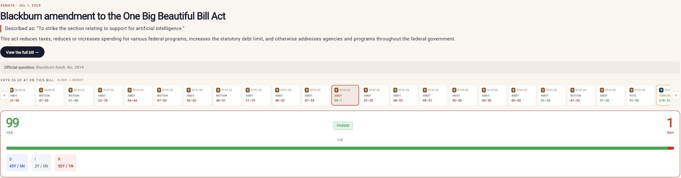
The amendment and final passage are separate decisions in the same legislative sequence.
1. What are we asking the model to predict?
The model predicts how each member will vote on a specific question. Those predictions produce two views in StringTheory—an expected vote tally and a list of members most likely to break with their party.
Step 1. Identify the question Congress is voting on.
A bill can come up for several votes before it passes or fails. Those votes can ask very different questions. Take the One Big Beautiful Bill Act.
Pass the bill? On final passage, a Yea supports passing that version of the bill in that chamber. A Nay opposes passing it. On July 1, senators split 50–50, and the vice president broke the tie. Final vote
Change the bill? An amendment proposes a change to the text. Earlier that day, senators voted 99–1 to remove the restriction on state AI regulation. A Yea supported removing that provision. Amendment vote
Take the next step? A procedural vote decides how the chamber handles the proposal. For example, a motion to proceed asks whether to begin considering a bill. A member can support taking it up, then oppose passing it.
Someone could therefore support removing the AI restriction and still oppose the rest of the bill. The model needs the exact question, the version of the text being considered, and whether the vote is in the House or Senate.
The wording of that question can even reverse what Yea means. A Yea to adopt an amendment supports making the change. A Yea to table it supports setting it aside.
The same preference about an amendment can imply opposite votes on adoption and tabling.
Earlier versions sometimes carried the bill’s expected support over to an amendment, or treated a Yea on tabling as support for the change. Those misses led us to identify the amendment and the action being voted on explicitly.
Step 2. Estimate each member’s choice.
For that specific vote, the model assigns each member a chance of Yea, Nay, or not voting. An illustrative prediction could be 70% Yea, 25% Nay and 5% not voting. These are probabilities, so they add up to 100%.
It also estimates the chance of a defection—voting against most members of one’s own party. On the July 1 final vote, most Republicans voted Yea, so the three Republican Nays counted as defections. The Democratic Nays followed their party’s majority. Before a vote happens, the model must estimate that party position too, in order to estimate defection likelihood.
Step 3. Combine the predictions into what you see in the app.
Adding the members’ Yea probabilities gives the expected number of Yeas across all members. We do the same for Nays and non-voters. Adding their defection probabilities gives Expected Defections, while Defection Watch highlights the members most likely to break with their party.
That gives us a clear job for the model. Identify the decision, estimate each member’s response, and combine those estimates into a picture of the chamber. We can then estimate whether the proposal will clear the threshold to pass. The next section introduces the information used to make these predictions, called features.
2. What does the model use to predict?
For each member and decision, the pipeline assembles a feature vector—a list of numbers describing the member and the decision, using information available before the vote. It combines prior attendance and voting behavior, ideology, sponsorship and cosponsorship, committee relationships, political cross-pressure, available financial signals, and the procedural context we just defined in section 1.
Some inputs describe the member. Others describe the member’s relationship to this particular decision. Sponsoring an amendment is more specific evidence than belonging to the party that introduced the parent bill. A record of crossing party lines on one policy area may tell us more than a single career-wide defection rate.
One of the hardest parts of building a historical forecast is preventing the model from seeing what happened afterward. This is data leakage. It can make a model look accurate by giving it clues a forecaster at the time could never have used.
First, set an information cutoff for the vote.
Before the July 1 AI amendment vote, its 99–1 result is unavailable. Once that result is recorded, it can inform the later final-passage forecast. The final 50–50 result stays outside the inputs for predicting final passage. Amendment vote · Final vote
This is sequential updating. New evidence can change the next forecast, while each forecast keeps its own cutoff. The checks reject inputs containing the target vote’s recorded tally or actual party-majority positions. Earlier roll calls are checked against the target’s identity, date and, where available, timestamp or roll-call order.
Then, check when each source became available.
Suppose a lawmaker receives a donation on June 1, votes on June 15, and first reports the donation publicly in July.
The June 15 forecast excludes that donation. The money had arrived, but the public record did not yet show it. A forecast can use only donations that were already made and publicly disclosed before the vote. If we cannot establish when a donation became public, we leave it out of that forecast too.
Once the July filing arrives, a separate historical analysis can include the donation to reconstruct the lawmaker’s funding before the vote. That analysis uses information learned later, so we keep it separate when measuring how well we could have predicted the June 15 vote.
Apply the cutoff to summaries too.
Today’s bill text may contain changes adopted after the vote. An ideology score calculated from an entire Congress may already reflect the vote we are trying to predict. The pipeline resolves the bill version available at the cutoff and uses earlier-Congress ideology statistics. Every summary needs the same scrutiny as the records behind it.
Some records give only a calendar date. A June 15 sponsorship can enter a forecast for a June 15 vote only when a timestamp or recorded sequence establishes that it came first. Records whose pre-vote availability cannot be established stay outside that forecast.
Even information that passes these timing checks has to prove useful. We can test that by comparing two sets of predictions for the same later votes—one using the information and one leaving it out—and checking which makes fewer mistakes.
The next step is to use the connections already stored in StringTheory’s knowledge graph. Members connect to the bills they sponsor and the votes they cast. Campaign-finance records connect those same members, through their campaign committees, to contributors and PACs. Following these links brings together a member’s voting history, funding sources, and the other members who share donors or support the same legislation. Relational deep learning is designed to learn patterns across records connected in this way.
3. Learn from connected records with Relational Deep Learning
Relational deep learning uses neural networks to learn from both the information in records and the connections between them. StringTheory already organizes congressional evidence this way. Members connect to the bills they sponsor and the votes they cast. Each vote connects back to the legislation being decided. Campaign-finance records connect members to donors through their campaign committees, while outside-spending records identify groups supporting or opposing them. These links let us trace shared sources of financial support across members.
Consider the One Big Beautiful Bill Act. A member’s earlier voting record and the bill’s sponsorship pattern each provide context. Linking them lets the model examine combinations, such as how members with a particular voting history behave on bills with support from both parties.
Kumo AI helped develop relational deep learning into tools for making predictions from connected business data. Its research developed relational foundation models, pretrained models that use related tables and examples with known answers to make predictions on new data. NVIDIA’s acquisition of Kumo was reported in June 2026. NVIDIA now provides downloadable model weights and open-source software for running these models, giving builders like me a model that has already learned how to find patterns across connected records. KumoRFM-2 research · Acquisition reporting · NVIDIA Kumo
StringTheory uses NVIDIA’s Kumo-Relational, a pretrained relational foundation model built on the KumoRFM-2 architecture—the neural-network design shown below. I’ll call this pretrained model Kumo throughout the article. NVIDIA trained it on synthetic databases—computer-generated tables and relationships—progressing from single tables to more complex linked data. We supply the congressional context by giving it member and bill records, their connections through earlier votes, and examples of whether members defected. This lets it apply what it learned during pretraining to the voting patterns in our data. NVIDIA’s model explanation · Model card
The diagram below shows how those capabilities fit together. Its example links users, orders and items. The same operations can work on members, votes and bills.
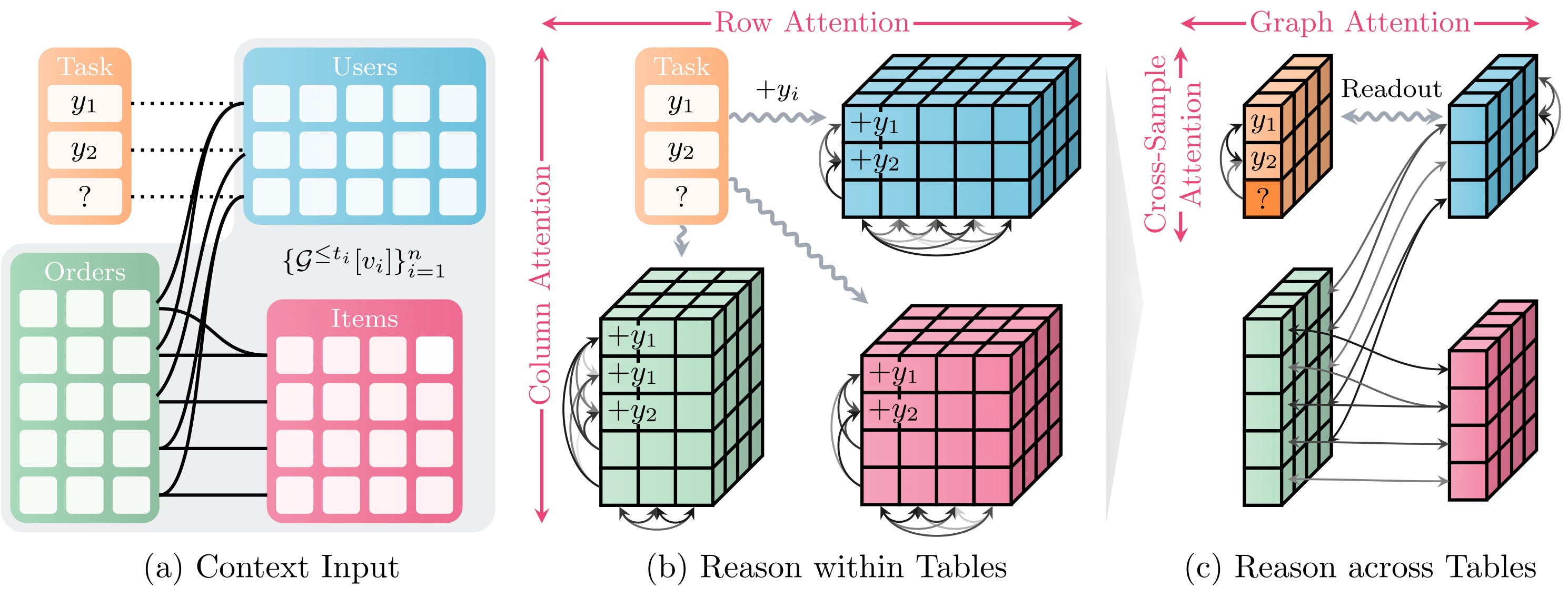
Read panels (a), (b) and (c) from left to right. The question mark is the outcome to predict. The arrows show how information moves within tables and across their links.
Figure 3 by Hudovernik et al., KumoRFM-2: Scaling Foundation Models for Relational Learning, reproduced under CC BY 4.0.
In our July 1 example, the question is whether a senator will defect on the final vote. Follow that case through the diagram.
Give it past examples, panel (a). We supply earlier votes, the connected member and bill records, and whether each member defected. These are the known answers in the diagram. For the July 1 case we want to predict, we leave the answer blank.
Summarize each record, panel (b). Kumo combines the information within each table, giving different pieces different weight. This is attention. It turns each record into a numerical summary called an embedding. The senator’s summary reflects their available voting history. The bill’s reflects its sponsorship data. Graph attention explained · Node embeddings explained
Connect the person to the decision, panel (c). The model follows the links from the vote scenario to its senator and bill, then combines their embeddings. The case now describes this person facing this legislation. Passing information between connected records is called message passing. A visual guide to message passing
Use the known cases to make an estimate, panel (c). It then weighs the earlier examples for their relevance to the new case, then produces a probability of defection. The examples guide its answer while its pretrained weights—its learned settings—stay fixed. This is in-context learning. How Kumo uses examples
We currently use three linked tables from StringTheory’s broader graph as input to Kumo.
Members carry historical measures such as ideology, attendance, party loyalty and defection rate.
Bills carry measures such as the number of cosponsors and how bipartisan that sponsorship is.
Member–vote examples identify the member and bill, the expected party position, and whether the member sponsored the legislation. The member and bill IDs connect each example to the other two tables.
Our examples with known answers come from individual members’ votes in the 114th–117th Congresses. Each includes the member and bill information plus whether that member defected. We supply these examples when we run Kumo, so it can use those past cases to interpret the new case.
We also set how far Kumo can follow the graph connections. In this version, it follows two links from each prediction question. The first leads to the member–vote record. The second leads from that record to the member or the bill. This brings a summary of the member’s earlier voting and the bill’s sponsorship information into the same calculation.
The embeddings from Kumo summarize these legislative tables. Campaign-finance information enters through separate numerical features alongside the embeddings and prediction scores. Feeding contributor and contribution records directly into Kumo is an experiment we will be running, explained in the last section.
I keep two outputs from Kumo.
An embedding. This is a list of 512 numbers describing patterns in the connected records. Our code compresses it to an eight-number embedding for each saved profile using singular value decomposition, or SVD. This keeps eight combinations that capture the largest differences across the embeddings. Each saved number combines information from many original dimensions.
An initial defection probability. Kumo uses the known examples to estimate how likely a member is to depart from the expected party position. Our code turns this probability into prediction scores for the next stage. It adjusts the defection score using the member’s earlier defection rate and the current vote’s context, then calculates a Yea score using the expected party direction.
I save the compressed embeddings and prediction scores in a cache, a file the forecasting pipeline can reuse. For a new member–vote case, our code combines the saved member and bill embeddings into an eight-number embedding and prepares the Yea score and defection score. It also compares the member and bill embeddings to calculate a member–bill alignment score. These are the inputs we pass to the congressional models.
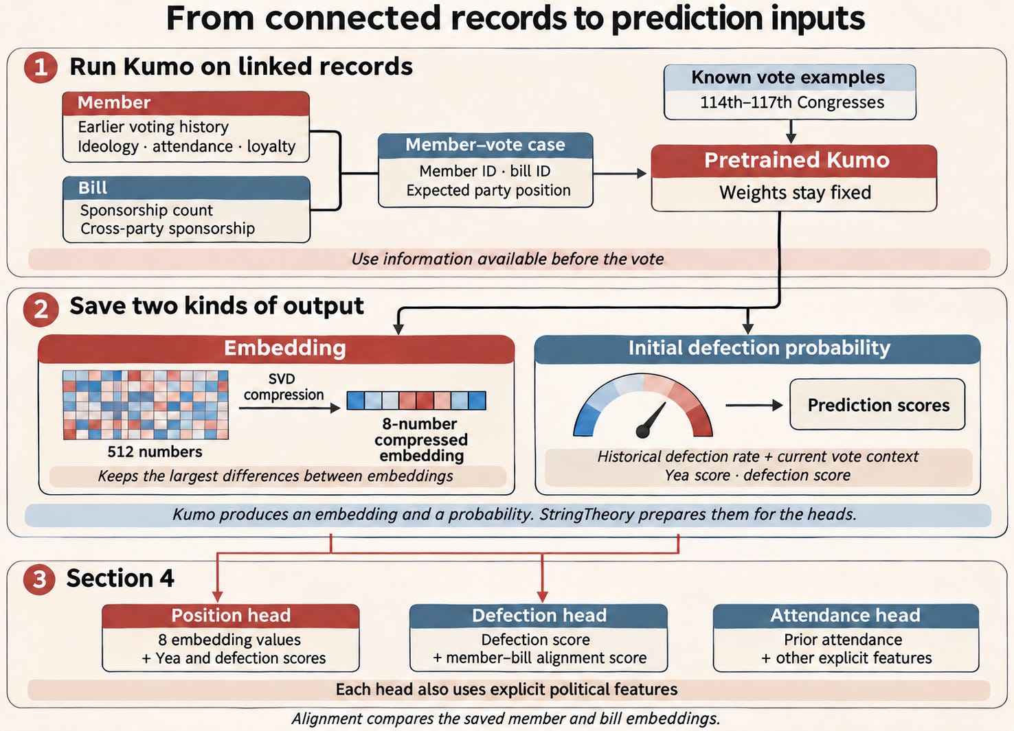
StringTheory uses Kumo’s two outputs—an embedding and an initial defection probability. Our pipeline compresses the embedding and adjusts the probability into prediction scores for the congressional models. The colored cells illustrate the numbers in an embedding.
The information cutoff from section 2 applies to the cached embeddings and prediction scores too. The cache selects member profiles by Congress, uses earlier-Congress statistics and builds vote-specific sponsorship counts from records available before the vote.
We now have compressed embeddings and prediction scores for each member–vote case. The next step is to train the congressional models that use these inputs.
4. Train the congressional prediction heads
A prediction head is a small model trained to answer one question. It learns how to combine its inputs by training on earlier member–vote cases with known outcomes. We train three heads for the questions from section 1.
First, we need the party position that a member might depart from. A separate caucus model estimates whether most Democrats and most Republicans will vote Yea or Nay, and how certain those estimates are. It uses procedure, sponsorship, available committee evidence and earlier relevant votes. The position and defection heads receive the expected party position as an input.
Attendance head—will the member participate? It uses directly calculated features, including earlier attendance and the vote’s expected closeness.
Position head—if the member participates, how likely are they to vote Yea? It receives the eight-number Kumo embedding, the Yea and defection scores, and directly calculated political features.
Defection head—how likely is the member to depart from the expected party position? It uses the defection score and member–bill alignment score alongside directly calculated political features.
These directly calculated inputs are our explicit features. They describe the member’s history, the decision being made and the sequence of events leading up to it.
Member history. Prior attendance, ideology, bipartisanship and defection rates describe the member’s earlier behavior. Ideological distance from the party provides another measure of how typical that member is.
The decision at hand. The expected party position, type of motion, sponsorship, and level of cross-party cosponsorship describe the particular vote. An amendment sponsor and a member voting on final passage can therefore receive different inputs.
The sequence so far. Earlier same-bill votes, the member’s recorded position on those votes, and the available bill-version history provide evidence about how support is developing.
In the July 1 example, the same senator appears in both the amendment vote and final passage, but the motion and the available earlier-vote evidence change. These explicit inputs let the heads respond to that difference alongside the embedding and prediction scores.
The position and defection heads also use finance summaries, including PAC support relative to fundraising and a member’s donor-industry alignment compared with their party. These turn eligible financial records into numerical inputs that the heads combine with political history, embeddings and prediction scores. Records must pass the disclosure-date and coverage checks before contributing to the forecast.
During training, we give each head the information available before an earlier vote, then compare its prediction with what actually happened. A loss function measures the error. For example, assigning a 20% chance of Yea to a member who voted Yea produces a larger probability error than assigning 80%. An optimizer adjusts the head’s weights—the settings that determine how it combines inputs—to reduce error across the training cases.
We train the attendance and position heads first. We then hold them fixed while training the defection head, which learns to refine the defection estimate implied by the position head. Kumo’s pretrained weights stay fixed throughout.
The main historical split uses the 114th–117th Congresses for training, the 118th for development and calibration, and later 119th Congress records for evaluation. The pipeline also uses curated, feature-rich training examples. Each evaluation identifies the records used for fitting and the examples that have already influenced development.
The loss function tells the model which mistakes to correct during training. Suppose 100 members are voting, and 95 follow their party while five defect. Predicting that everyone follows their party would be 95% accurate, yet miss all five defectors. The loss function needs to make those missed defections costly, even when most other predictions are correct. We therefore train the position and defection heads against four kinds of error.
Individual probability error. Confidently assigning the wrong vote carries a penalty. Focal loss reduces the influence of already-easy examples so harder cases receive more attention.
Party-level count error. The model is also penalized when its expected support within a party misses that party’s recorded support. Individually plausible probabilities can still add up to a poor coalition estimate.
Repeated member-level bias. Across a member’s training history, expected and recorded defections are compared. This discourages systematically treating the same person as more or less independent than their record supports.
Ranking error. The defection objective rewards placing actual defectors above non-defectors on the same roll call. A watchlist needs the right names near the top.
The final Senate vote on the One Big Beautiful Bill Act illustrates why all four matter. A forecast could get the number of Republican Nays right while selecting the wrong three people. It could identify one likely dissenter but underestimate the whole group. Those are different failures, and the training objective needs to expose both.
Once training is complete, the heads turn a new member–vote case into three scores, expressing how strongly the learned evidence points toward participation, Yea and defection. Our current forecasting pipeline uses those scores as corrections to a starting forecast built from political rules. The next section follows one prediction through that calculation.
5. Combine and calibrate the forecast
The starting forecast comes from hand-written rules about party support, the type of vote and the member’s record. Consider a hypothetical senator whose party is expected to support a bill. Those rules might give the senator an initial 80% chance of voting Yea, assuming they participate.
We then use the heads trained in section 4 to work out how that estimate should change.
Score the senator with the full inputs. The trained heads receive the relevant embeddings, prediction scores and explicit features described above. Their outputs express the learned evidence for this senator on this vote.
Calculate a comparison score. We make modified copies of the trained heads, called reference heads. These copies remove the eight embedding values and both prediction scores from the position head, and the defection score from the defection head. They also slightly reduce some of the remaining weights. We run the same senator–vote case through them. This tells us how the scores change when we move from that simpler model to the full one.
Turn that difference into a correction. Suppose the full position head favors Yea less strongly than the reference does. That difference pushes the initial Yea estimate downward. Both heads can favor Yea, while the comparison still provides a reason to lower the original 80%.
The full-input heads could supply the member probabilities directly. Our current design adds the comparison because it keeps a separate, rule-based starting forecast and uses the learned model to adjust it.
Here is the extra information the second prediction provides. Suppose the full position head gives our hypothetical senator a 70% chance of Yea.
If the reference gives 90%, the full model has become less supportive of Yea. The comparison shows a shift toward Nay.
If the reference gives 50%, the full model has become more supportive of Yea. The comparison shows a shift toward Yea.
The full model gives the same 70% in both examples. The reference tells us which way the model’s answer changed. That change is what this pipeline uses to revise the political starting forecast. These percentages illustrate the direction of the model’s change. The calculation applies weights to differences in the underlying scores.
The practical benefit is control over how much a learned change affects the final forecast. We can retain an explicit rule about the decision being voted on, then let learned member–bill patterns adjust individual predictions. We also weight a change shared across a party separately from one that makes a single member stand out. A small shift affecting hundreds of members can otherwise produce a large change in the expected tally.
That control comes with a tradeoff. It can restrain a mistaken model signal, but it can also hold back a correct signal when the political starting estimate is wrong. Using the full heads directly gives their probabilities more influence over the result. The accuracy benefit of our comparison-based approach needs to be measured against that alternative. Section 7 describes the test.
The senator’s defection probability also depends on which way most of their party will vote. The caucus model from section 4 supplies that estimate. Suppose it gives the party an 80% chance of mostly voting Yea and a 20% chance of mostly voting Nay.
First, assume the party mostly votes Yea. Estimate the senator’s vote under that assumption. A Nay would count as a defection.
Then, assume the party mostly votes Nay. Estimate the senator’s vote again. This time, a Yea would count as a defection.
Combine the two predictions. Give the first scenario 80% of the weight and the second 20%, following the caucus model’s estimate.
The result carries both uncertainties into the forecast—how the senator will vote, and whether that choice will put them on the opposite side of most of their party. This matters most when the party could split closely enough for its majority position to change.
Getting the party’s direction right can still miss the tally
We also need to estimate how many members will depart from that direction. The House vote on the GENIUS Act makes this problem concrete. It passed with 308 Yeas and 122 Nays.
Democrats split 102 Yea to 110 Nay. Their majority opposed the bill, but almost half supported it. Those 102 Yeas counted as defections.
Republicans split 206 Yea to 12 Nay. Their majority supported the bill. Those 12 Nays counted as defections.
That makes 114 defections. A forecast could correctly expect a Democratic Nay majority and a Republican Yea majority while still missing much of the bill’s support. It has to distinguish a handful of Democratic crossovers from the 102 who actually voted Yea. Recorded House vote
The model’s historical replay estimates 208.5 Yeas, falling 99.5 short of the recorded 308. For this comparison, the app scales its expected Yea and Nay counts to the 430 members who actually cast one of those votes.
Recognizing a party’s majority position is only part of the task. The model must also estimate how many members will cross over. On GENIUS, 102 Democrats supported the bill even as most of their party opposed it.
Misses like this led us to give the model more detail about coalition patterns. It distinguishes different kinds of party support, looks at sponsorship within the chamber that is voting, and can use earlier votes on the bill. Each is a way to identify support that extends beyond the usual party division. The GENIUS result shows that these additions still leave a large gap. Section 7 returns to ways to test richer evidence and give learned coalition shifts more influence.
The probabilities also need to match how often defections actually happen. That is calibration. Across many member–vote cases assigned a 20% defection probability, we want roughly one in five to be an actual defection. Probability calibration explained
Small probability errors add up. If 50 members each receive a 10% defection probability, the forecast expects five defections. If cases like these produce only two on average, the forecast systematically overstates dissent—even if it puts the most likely defectors at the top of the list.
Adjusting confidence at two different points
Two calibration steps operate at different points. During development, we tune how confidently the position head expresses its predictions. When generating a forecast, we check how much dissent the combined member predictions imply for each party.
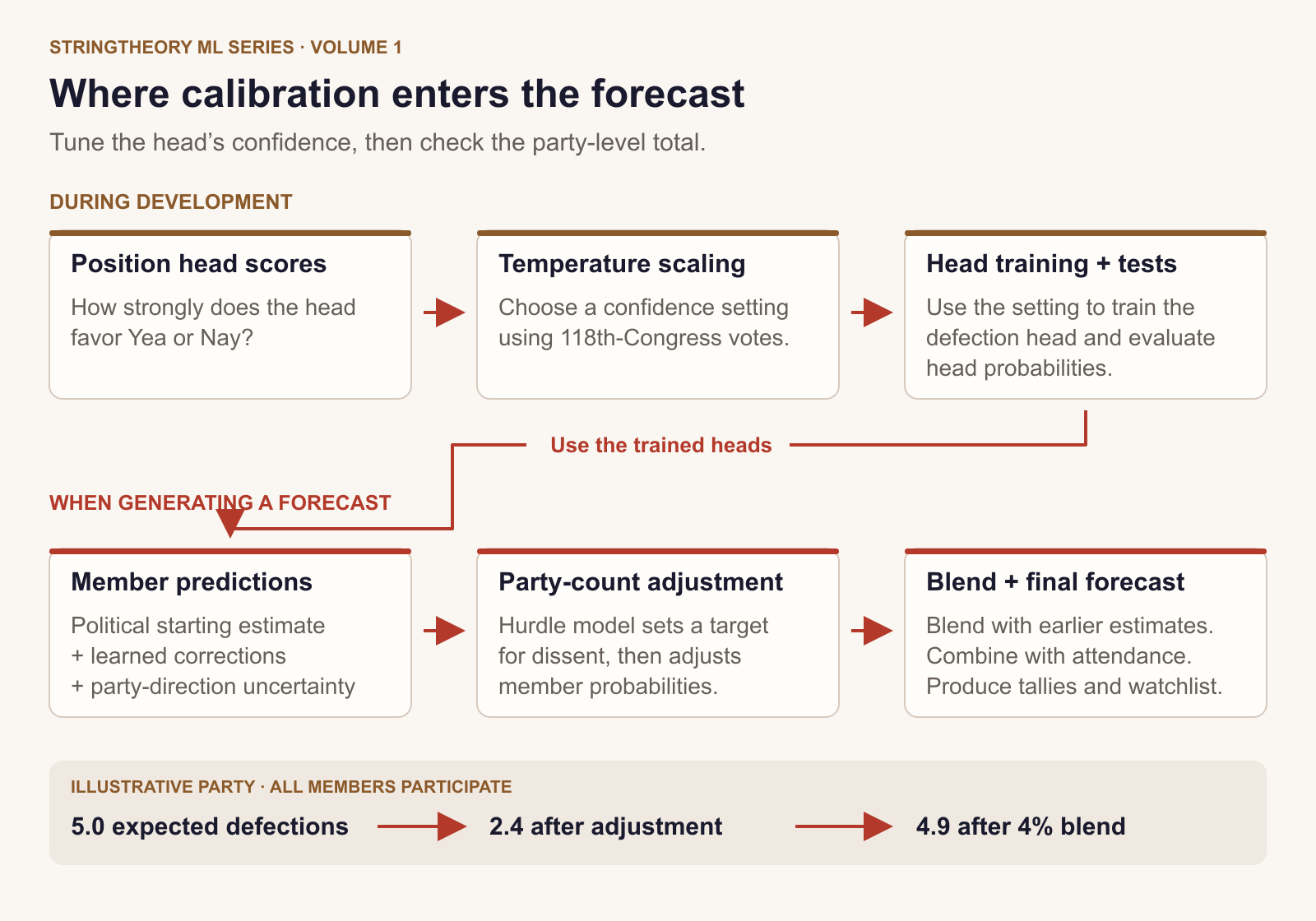
The confidence setting helps train and evaluate the heads. The live forecast then adjusts the party-wide amount of dissent and blends that adjustment into the member predictions.
First, tune the position head’s confidence
Temperature scaling applies one shared setting to the position head’s scores before converting them to probabilities. Suppose the head is too hesitant. An illustrative setting could move a 60% Yea estimate to about 69% and a 40% estimate to about 31%. The head still favors the same side in each case, but expresses that preference more strongly.
We choose the setting using votes from the 118th Congress. We try several settings and select the one with the lowest log loss across those examples. This score penalizes a confident wrong prediction more heavily than a cautious wrong one. How temperature scaling works
That setting is used when training the defection head and evaluating the heads. The live forecast uses the trained heads through the starting-estimate-and-correction calculation described above.
Then, check the expected size of each party’s split
We use a separate fitted component here, called the hurdle calibrator. It comes after the member predictions and adjusts how much dissent they imply for each party. The three parts have different jobs.
The caucus model estimates which side the party’s majority will take. For example, will most Democrats vote Yea or Nay?
The prediction heads estimate each member’s attendance, vote choice and likelihood of defection. We combine their full-input and reference scores with the political starting estimate, as described above.
The hurdle calibrator takes those member predictions and information about the vote, then estimates how much dissent to expect across the party.
The reason for adding this step is that the member probabilities can add up to the wrong amount of dissent, even when they identify the likeliest defectors. The GENIUS example shows the distinction. Expecting most Democrats to vote Nay still leaves the question of whether 10 Democrats or 102 will vote Yea. That difference can change the chamber forecast substantially.
The hurdle calibrator addresses this group-size question using patterns fitted from pre-119th-Congress roll calls, rules about the type of vote and the existing member predictions. Here is how it changes the forecast.
Estimate how likely the party is to stay together. Some votes produce almost no dissent. Others divide the party. This asks how tightly members vote together. The earlier caucus model estimated which side their majority would take.
Set an expected defection count. Consider an illustrative party of 50 members, all participating. Suppose the model assigns an 80% chance to a nearly united vote, with 0.5 expected defections, and a 20% chance to a split, with 10 expected defections. Weighting those possibilities gives 0.8 × 0.5 + 0.2 × 10 = 2.4 expected defections. A fractional count represents an average across possible outcomes.
Adjust the member probabilities toward that count. The calibrator raises or lowers their defection probabilities together. It preserves their order within the party, so a member rated more likely to defect stays above one rated less likely. The adjustment changes the overall amount of dissent those probabilities imply.
Blend with the earlier member estimates. For most votes, the current pipeline gives the earlier estimates 96% of the weight and the count-adjusted estimates 4%. In our all-participating example, an earlier total of five defections and an adjusted total of 2.4 would produce about 4.9 expected defections after blending. Certain cloture votes—votes to end debate—use the full adjustment under separate rules.
This explains why the calibrator’s target can differ from the final forecast. Its influence depends on the blend. A small weight preserves more of the earlier member predictions, but also limits how much the calibrator can correct a mistaken party total. Section 7 includes testing how strongly learned evidence should change the forecast.
We keep the final Yea, Nay and non-voting probabilities consistent, then add them up for the chamber and rank members for Defection Watch. Section 6 tests whether those final probabilities match what happens on later votes, after all the adjustments.
Turning probabilities into a chamber forecast
After combining attendance and position, a hypothetical member with a 96% participation probability and a 70% conditional Yea probability has 67.2% Yea, 28.8% Nay and 4% not voting. Summing the final member probabilities produces expected chamber counts. Summing the defection probabilities produces Expected Defections.
Passing the chamber requires the forecast to clear the vote’s threshold. We estimate that probability while allowing for uncertainty in how many members vote Yea. The present system includes an approximate allowance for members moving together, such as several members of a faction changing position at once. Section 7 returns to the challenge of modeling that shared movement on close votes.
6. Evaluate the forecasts
The final probabilities have to answer three questions. Do they express uncertainty honestly? Do they put likely defectors near the top of the watchlist? Do they add up to a useful estimate of the vote’s outcome?
Start with a fair comparison
This particular test evaluates vote choice among members who actually participated. It measures how well we predict their choices and the resulting counts. Attendance forecasting needs its own evaluation.
We compare StringTheory with a simple sponsor-party and ideology baseline. It expects members of the sponsor’s party to support the proposal and adjusts that expectation using their ideological distance from the sponsor. Both forecasts face the same votes and members. This gives us a concrete starting point for comparison.
Do the probabilities reflect what happens?
A 70% prediction should succeed about seven times in ten across comparable cases. Section 5 described how we adjust confidence. Here we measure the probabilities after those adjustments.
One measure is the Brier score, the average squared gap between a probability and the outcome. If we predict 70% Yea, a recorded Yea produces an error of 0.09 (0.3 squared) and a Nay produces 0.49 (0.7 squared). Lower scores are better. StringTheory scores 0.060, compared with 0.290 for the baseline.
A Brier score of zero would mean every prediction was certain and correct. Giving every vote a 50–50 chance would score 0.250. Our score of 0.060 therefore shows that the probabilities carry useful information about the outcomes. Compared with the baseline’s 0.290, they produce about 79% less squared prediction error across this test sample.
We also check whether the model’s confidence matches how often its favored answer is right. We group predictions with similar confidence and compare each group’s average confidence with its actual accuracy.
For example, suppose the model gives its chosen answer—Yea or Nay—an average of 80% confidence in one group. If those answers are correct 74% of the time, the model is overconfident by six percentage points in that group. If they are correct 86% of the time, it is underconfident by six points. Both count as a six-point gap.
Our 5.6-percentage-point average gap means the distance between stated confidence and observed accuracy averages 5.6 points across these groups, giving more weight to groups with more predictions. The baseline’s gap is 23.1 points. Individual groups can have larger or smaller gaps, so we examine them separately to see where the model expresses too much or too little confidence.
Does Defection Watch find the people who defect?
Top-10 recall asks what share of the actual defectors appear in the ten highest-ranked names. If eight members defect and four appear in the list, recall is 50%.
On the 115 roll calls in this sample that had at least one defection, the list finds an average of 35.6% of the actual defectors, compared with 6.5% for the baseline. We calculate that share separately for each roll call, then average the results.
Each roll call contributes equally to this average. Recall measures how much of the full group of defectors the watchlist captures.
The 35.6% recall means the top-ten list captures a little over one-third of the actual defectors on average across these votes. Roughly two-thirds remain outside the list. This is a substantial improvement over the baseline’s 6.5%, with considerable room to find more of the group.
Precision asks a different question. Of the people we flag, how many actually defect? If one member in a five-name list defects, its precision is 20%.
Among the five highest-ranked names, precision is 21.7% across the same 115 roll calls. That means an average five-name list contains about one actual defector and four members who follow their party. Even near the top of the ranking, many flagged members ultimately stay with their party.
The GENIUS Act shows why list length matters too. With 114 actual defectors, even a perfect ten-name list could find only 10 of 114, or 8.8%. A short list can identify its members accurately while covering only a small share of a large party split.
How close are the predicted totals?
We measure how far each predicted count is from the recorded result, then average those distances. This is mean absolute error. Predicting 52 Yeas when 49 members vote Yea gives an error of three. Predicting 46 against the same result also gives an error of three, so both contribute a three-vote error to the average.
Chamber size matters. With full participation, a 13-vote miss amounts to about three percentage points of the 435-member House and 13 points of the 100-member Senate. Comparing the chambers calls for separate averages and an error measured as a share of the members participating in each roll call. The combined figures below summarize both chambers together. A 13-vote miss can still change the outcome of a close vote in either chamber.
Across the 180 roll calls, the average Yea-count error is 13.8 members, compared with 36.5 for the baseline. The Yea estimate falls within three votes of the result on 52.2% of roll calls. For the total number of defections, the average error is 15.5 members, compared with 33.3 for the baseline.
Errors shown here combine both chambers. A given vote-count error represents a larger share of the Senate than of the House.
The 13.8-member Yea-count error means the forecast was about 14 votes away from the recorded Yea tally on average. That is roughly 62% less average error than the baseline. Individual forecasts can be much closer or much further away.
The 52.2% within three votes result makes that variation clearer. Just over half the forecasts landed within three votes of the recorded tally. Nearly half missed by more than three, and larger misses pull up the average error.
The 15.5-member defection-count error means the predicted number of defectors was off by about 16 members per roll call on average. That roughly halves the baseline’s error, but leaves substantial uncertainty about the size of a party split. Errors of this size matter especially when a bill’s outcome depends on a handful of votes.
Calibration matters beyond forecasting too. Suppose a member takes a particular position in 80 of 100 comparable cases. Predictions of 60% each imply 60 expected occurrences and an apparent 20 above expected. Predictions of 80% imply 80 expected occurrences and zero above expected. Both sets make the same yes-or-no calls, but they tell very different stories about unusual behavior.
For the historical split described in section 4, the prediction heads learn from the 114th–117th Congresses, and we use the 118th for development and calibration. The results above cover 180 roll calls from the 119th Congress, excluding 19 cases used during development. We reconstruct each prediction using information available before that vote, then compare it with the recorded outcome. Measuring forecasts saved before future votes will add a real-time test, with each prediction fixed before its outcome is known.
Across these tests, StringTheory improves on the baseline in probability accuracy, finding defectors and estimating vote totals. The remaining errors point to two priorities. We need to identify more of the members who will cross party lines, particularly in the House where bills like the GENIUS Act draw large cross-party coalitions, and better estimate how large those groups will become. Section 7 examines specific misses and the additional evidence that could help address them.
7. What the remaining misses can teach us
Each iteration on this and other models starts with missed predictions. We inspect the evidence available at the time, identify a possible cause and test a targeted change on other votes. The next round focuses on public statements, richer financial connections and how the model handles unfamiliar coalitions.
Capture what members say about the bill
On the final Senate vote, Susan Collins and Thom Tillis both voted Nay. The app’s historical replay assigns Collins a 29% Nay probability and Tillis 8%. It recognizes more uncertainty around Collins, but still expects both members to support the bill.

All three members shown voted Nay. The forecast expected each to vote Yea, with substantially more uncertainty around Collins.
Tillis had publicly opposed the bill three days earlier, citing Medicaid funding, hospitals and rural communities in North Carolina. That statement gives evidence about this bill that a general party-loyalty score can miss. Tillis’s June 28 statement
We’re connecting dated statements, floor speeches, letters and caucus endorsements to the exact bill, version or amendment. The model must distinguish firm opposition from conditional support, and recognize when a last-minute amendment compromise changes the coalition.
We’re also testing dissent from both ideological wings. A member can oppose a bill because it goes too far or because it does too little. Ideological direction and a member’s history of such rebellions may reveal holdouts that a single distance from the party center misses.
Give Kumo more of the financial graph
Kumo currently sees the legislative tables, while campaign-finance summaries reach the prediction heads separately. Those summaries can hide differences. In a hypothetical GENIUS Act comparison, two members might receive the same share of funding from finance, but one’s donors work in stablecoins and the other’s in insurance.
We’re testing linked donor, contribution, committee and member records, including outside spending for or against a member. We will compare following two versus three graph links, then add stock disclosures and more precise lobbying-to-bill connections. Comparing summaries and graph inputs built from the same records will show what their relationships add. Each record retains its pre-vote disclosure cutoff.
These details may help identify an unfamiliar coalition before the first roll call reveals who supports the bill.
Keep more of the embedding
Compressing Kumo’s 512-number embedding to eight numbers can discard patterns that matter for rare defections. We’re comparing eight, 32, 64 and all 512 numbers, retraining the heads for each version. The compression is fitted using training records. We will compare retained information, defector rankings, calibration and tally errors alongside cache size and scoring speed.
Let unfamiliar coalitions change the forecast
The GENIUS miss raises another question. Does the political starting estimate hold the forecast too close to the usual party split? I want to compare that starting estimate alone, the full prediction heads used directly, and our current correction approach. We will also vary how strongly the party-count adjustment changes the result.
Members can also move together after a negotiation or caucus decision. We’re testing shared movement within party and issue groups, and checking the forecast’s uncertainty. For example, an 80% range for the final tally should contain the result about eight times in ten. That check matters especially on close votes, where a small coordinated shift can change who wins.
Alongside these experiments, we’re improving the explanations shown for each member. Readers should be able to see which inputs moved the forecast and how those inputs relate to the underlying records.
For each experiment, we choose settings on development data and judge the final version on separate later votes. An improvement should help us find defectors, estimate coalition size or express uncertainty more accurately.
How to explore the forecasts and share feedback
You can explore forecasts on the Docket page or Rollcalls page, open a member’s record, and compare the prediction with the available evidence. Some full app views require sign-in. Send a revealing miss through Feedback or leave it in the comments—I’d like to examine it in a future installment.
This is the first model deep dive in the series, and I’d like your feedback on the format. Which examples or diagrams helped? Where did I lose you, and where would you like more technical detail? Tell me in the comments.
I’ll revisit these models in future volumes as upgrades ship, with before-and-after results, fresh test cases and a look at which misses we’ve fixed—and which still need work. Subscribe to follow those updates.
Thanks for reading and helping me shape this series.
— Pravin
P.S. Join me here on Substack tonight for our election live blog at 7 p.m., open chat at 8 p.m. and livestream at 9 p.m. All times ET.
Explore StringTheory: Web app · Android app